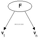
ï The algorithm operates over a set of training instances, C.
ï If all instances in C are in class P, create a node P and stop, otherwise select a feature F and create a decision node.
ï Partition the training instances in C into subsets according to the values of V.
ï Apply the algorithm recursively to each of the subsets C .
size: small medium large
colour: red blue green
shape: brick wedge sphere pillar%% yes
medium blue brick
small red sphere
large green pillar
large green sphere%% no
small red wedge
large red wedge
large red pillar
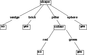
This can eaily be expressed as a nested if-statement
if (shape == wedge)
return no;
if (shape == brick)
return yes;
if (shape == pillar)
{
if (colour == red)
return no;
if (colour == green)
return yes;
}
if (shape == sphere)
return yes;
ï ID3 uses entropy to determine the most informative
attribute.
![]() (all
logs are base 2)
(all
logs are base 2)
ï Frequency can be used as a probability estimate.
ï E.g. if there are 5 +ve examples and 3 -ve examples in a node the estimated probability of +ve is 5/8 = 0.625.
ï Work out entropy based on distribution of classes.
ï Trying splitting on each attribute.
ï Work out expected information gain for each attribute
ï Choose best attribute
ï There are 4 +ve examples and 3 -ve examples
ï i.e. probability of +ve is 4/7 = 0.57; probability of -ve is 3/7 = 0.43
ï Entropy is: - (0.57 x log 0.57) - (0.43 x log 0.43) = 0.99
ï Evaluate possible ways of splitting.
ï Try split on size which has three values: large, medium and small.
ï There are four instances with size = large.
ï There are two large positives examples and two large negative examples.
ï The probability of +ve is 0.5
ï The entropy is: - (0.5 x log 0.5) - (0.5 x log 0.5) = 1
ï There is one small +ve and one small -ve
ï Entropy is: - (0.5 x log 0.5) - (0.5 x log 0.5) = 1
ï There is only one medium +ve and no medium -ves, so entropy is 0.
ï Expected information for a split on size is:
![]()
ï The expected information gain is: 0.99 ó 0.86 = 0.13
ï Now try splitting on colour and shape.
ï Colour has an information gain of 0.52
ï Shape has an information gain of 0.7
ï Therefore split on shape.
ï Repeat for all subtree
2. Use the induction algorithm to form a rule to explain the current window.
3. Scan through all of the training instances looking for exceptions to the rule.
4. Add the exceptions to the window
ï If S were replaced by a leaf, we expect the error rate to increase.
ï The complexity of S can be measured by the average path lengh from the root to the leaves.
ï C4 repeatedly finds the subtree, S, with the least ratio of increased error rate to complexity.
ï If it is significantly worse the the average over all subtrees, S is replaced by a leaf.
ï Approximate backed-up error from children assuming we did not prune.
ï If expected error isless than backed-up error, prune.
ï What will be the expected classification error
at this leaf?
![]()
S is the set of examples in a node
k is the number of classes
N examples in S
C is the majority class in S
n out of N examples in S belong to C
ï Let chidren of Node be Node1, Node2,
etc
![]()
ï Probabilities can be estimated by relative frequencies of attribute values in sets of examples that fall into child nodes.
![]()

![]()
ï Right child has error of 0.333
ï Static error estimate E(b) is 0.375
ï Backed-up error is
![]()