Figure 1: The "Internet Hourglass" (source: ICOM6012 Topic 3 Application Layer).
| Date | Version | Description |
|---|---|---|
| 24/02/2026 | 1.0 | Initial release |
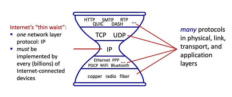
The Internet Protocol (IP) is the fundamental protocol that enables data to be sent across interconnected networks. It provides a global addressing scheme and a routing framework that allows packets to be delivered from a source host to a destination host, even across heterogeneous physical networks. By defining a common packet format and addressing system, IP creates a unifying layer that supports end-to-end communication between diverse devices.
Figure 1: The "Internet Hourglass" (source: ICOM6012 Topic 3 Application Layer).
An IP address is a numerical identifier assigned to a network interface. At the IP layer, addresses serve two primary roles:

Figure 3: Each IPv4 packet includes the source and destination address in the header for identification and forwarding.
Introduced in 1980, Internet Protocol version 4 (IPv4) remains the dominant protocol of the Internet. IPv4 uses a 32-bit address space, providing $2^{32}$ (approximately 4.3 billion) unique addresses. These addresses are typically written in the more human-friendly dotted-decimal notation, where each 8-bit byte (or "octet") is represented by its decimal value, ranging from 0 to 255, and separated by full stops. An example is provided in Figure 2.

Figure 2: An IPv4 address in both binary and dotted-decimal notation.
Not all IPv4 addresses are intended for general use. Large portions of the address space are reserved for special networking purposes. For example, the following ranges are reserved for private use:
| Address Range | CIDR Block | Number of Addresses |
|---|---|---|
10.0.0.0 $\to$ 10.255.255.255 |
10.0.0.0/8 |
$2^{24} = 16,777,216$ |
172.16.0.0 $\to$ 172.31.255.255 |
172.16.0.0/12 |
$2^{20} = 1,048,576$ |
192.168.0.0 $\to$ 192.168.255.255 |
192.168.0.0/16 |
$2^{16} = 65,536$ |
Addresses from these private ranges are not globally routable on the public Internet. Networks may use them internally as they wish, but packets containing private addresses are not forwarded across the public Internet.
Aside: CIDR Notation
CIDR (Classless Inter-Domain Routing) notation describes a contiguous range of IP addresses using an address and a prefix length that specifies how many leading bits are fixed.
For example, 192.168.1.0/24 fixes the first 24 bits (i.e., the 192.168.1 part) and represents $2^{32-24} = 2^{8} = 256$ consecutive addresses, from 192.168.1.0 to 192.168.1.255.
The first and last addresses in the range are obtained by setting the last $32-24=8$ bits to all 0s and all 1s, respectively.
Another example is the block 127.0.0.0/8 (i.e., 127.0.0.0 $\to$ 127.255.255.255), which is reserved for loopback.
Loopback addresses allow a host to send IP traffic to itself.
Such traffic is processed entirely within the operating system and never placed on a physical network, making loopback useful for testing and local inter-process communication.
Although this is a very large block of almost 17 million addresses, in practice only 127.0.0.1 is commonly used.
The global IPv4 address space is managed by the Internet Assigned Numbers Authority (IANA) and distributed via five Regional Internet Registries (RIRs).
The RIRs allocate address blocks within their respective regions, shown in Figure 4, to Internet Service Providers (ISPs), universities, governments, telecommunications companies, and other enterprises.
For example, the block 129.94.0.0/16 is managed by the Asia Pacific Network Information Centre (APNIC), the RIR for the Asia Pacific region.
APNIC delegated this block of 65,536 addresses to UNSW, hence when you're connected to a CSE machine you may notice its IPv4 address begins with 129.94.

Figure 4: Map of Regional Internet Registries (source: IANA).
Although a 32-bit address space appeared ample when IPv4 was designed, rapid Internet growth quickly led to concerns about address exhaustion. By 2011, IANA had allocated the last remaining blocks of unassigned IPv4 address space to the RIRs. Since then, most RIRs have exhausted their freely available IPv4 pools. Over the years APNIC has introduced various rationing policies to delay the point of exhaustion in its region, but we can see in Figure 5 that very few available addresses remain in the Asia Pacific.

Figure 5: Availability of IPv4 addresses in the Asia Pacific region (source: APNIC).
The long-term solution to IPv4 address exhaustion is the deployment of Internet Protocol version 6 (IPv6), which uses a 128-bit address space, providing a vastly larger pool of addresses. Deployment began in the mid-2000s and remains ongoing today, with adoption progressing gradually due to compatibility challenges and infrastructure costs.
In the meantime, Network Address Translation (NAT) emerged as a critical practical mechanism that has mitigated IPv4 scarcity for decades, enabling the continued growth of the Internet and playing a central role in modern network architecture.
Network Address Translation (NAT) is a technique used to translate IP addresses (and, in some cases, transport-layer identifiers) as packets pass between two different address realms:
A NAT device rewrites packet headers as traffic crosses the boundary between these two realms, and maintains state (a translation table) so that return traffic can be translated back correctly.
This allows internal addresses to have only local significance, enabling the same private IP address ranges to be reused across millions of independent networks worldwide while maintaining connectivity to the public Internet.
Traditionally NAT refers to one of two variants: Basic NAT and Network Address Port Translation (NAPT).
Basic NAT performs a one-to-one mapping of IP addresses, where each internal host that needs to communicate with the outside world is assigned a dedicated external IP address. This approach requires the NAT device to maintain a pool of public addresses; consequently, the number of internal hosts that can access the external network simultaneously is strictly limited by the size of that pool.
An example is illustrated in Figure 6. The internal network uses private addresses from the 10.0.0.0/8 IPv4 block and is connected to the public Internet via a NAT-enabled router. This router has access to a pool of public IPv4 addresses (e.g., 192.0.2.1 to 192.0.2.10).

Figure 6: An example of Basic NAT.
When the internal host 10.0.0.2 wishes to send a packet to the external server 203.0.113.1, the packet passes through the NAT-enabled router (1). The router checks its translation table for an existing mapping for 10.0.0.2. If none exists, it selects an available public address from its pool (e.g., 192.0.2.1) and creates a new mapping entry. The router then rewrites the source address in the IPv4 header using the mapped external address before forwarding the packet towards its destination (2).
Packets on the return path are addressed to 192.0.2.1 (3); the router consults the translation table and rewrites the destination address back to 10.0.0.2 before forwarding the packet to the internal host (4).
Translation table entries may be statically configured (permanent) or dynamically assigned (allocated from the pool as needed for the lifetime of the mapping).
While Basic NAT has practical use cases, its one-to-one mapping prevents it from scaling to solve IPv4 address exhaustion.
Aside: Documentation Addresses
The 192.0.2.0/24, 198.51.100.0/24, and 203.0.113.0/24 address blocks used throughout the examples are not actually globally routable. These blocks are reserved for documentation — that is, for use in examples in specifications and other documents, like this assignment. Using designated address ranges for documentation reduces the likelihood of conflicts or confusion that could arise from using addresses assigned for other purposes.
This practice isn’t unique to IP addresses. For example, reserved domain names such as example.com, example.net, and example.org exist for documentation, and various telephone numbers in many countries are also reserved for documentation, advertising, or fictional use.
Network Address Port Translation (NAPT) extends Basic NAT by translating not only IP addresses but also transport-layer identifiers, such as TCP and UDP port numbers. By multiplexing multiple connections using port numbers, NAPT allows many internal hosts to share a single external IPv4 address, with each connection distinguished by a unique port mapping.
An example is illustrated in Figure 7. As before, the internal network uses private addresses from the 10.0.0.0/8 IPv4 block and is connected to the public Internet via a NAT-enabled router. In this case, the router has a single external IPv4 address, 192.0.2.1.

Figure 7: An example of Network Address Port Translation (NAPT).
Suppose the internal host 10.0.0.2 sends an HTTP request to a Web server at IPv4 address 203.0.113.1, which listens on port 80. The host selects an arbitrary source port number, such as 5001, and sends the packet via the NAT-enabled router (1). Upon receiving the packet, the router checks its NAT translation table for an existing mapping. If none exists, the router allocates an unused external source port number (e.g. 1024) and creates a new translation table entry. The router then replaces the source IPv4 address 10.0.0.2 with its external address 192.0.2.1, and replaces the source port number 5001 with the mapped external port number 1024, before forwarding the packet towards the Web server (2).
The Web server, unaware that the packet has been modified by the NAT router, responds with a packet whose destination address is 192.0.2.1 and whose destination port number is 1024 (3). When this packet arrives at the NAT router, the router indexes its translation table using the destination address and destination port number to determine the corresponding internal host (10.0.0.2) and destination port (5001). The router then rewrites the packet’s destination address and port number accordingly, and forwards the packet to the internal host (4).
As with Basic NAT, translation table entries may be statically configured or dynamically assigned.
Because the port number field is 16 bits long, NAPT can support on the order of 60,000 simultaneous mappings per external IPv4 address, making it far more scalable than Basic NAT and the dominant form of NAT used in practice.
Technical Note: Some nuances of translation tables:
Aside: Home Networks
There is a very good chance the configuration in Figure 7 resembles your home network, where your ISP allocates a single public IPv4 address that is shared among multiple devices via a NAT device running in your home router. Though your internal network is more likely using private IPv4 addresses in the 192.168.0.0/16 block, rather than 10.0.0.0/8.
In some cases, the ISP itself may also deploy NAT — often referred to as carrier-grade NAT (CGN) — assigning non-globally routable IPv4 addresses to customers within its own internal network. This can create a hierarchy of NATs, with multiple layers of address translation between end users and the public Internet. The block 100.64.0.0/10 (i.e. 100.64.0.0 $\to$ 100.127.255.255) is reserved as “shared address space”. It is similar to the private address blocks, but is specifically intended for use by ISPs running CGN.
This assignment is focused on Network Address Port Translation (NAPT) over IPv4, but for simplicity, the broader terms NAT and IP are used throughout the remainder of the specification. All future references to NAT and IP should be interpreted as NAPT and IPv4, respectively.
In this assignment, you will implement a Network Address Translation (NAT) device in C, Java, or Python.
Your NAT will translate IP addresses and UDP port numbers as packets pass between an internal network and an external network.
Under certain conditions, your NAT will also generate appropriate ICMP error messages.
A real NAT operates within the operating system’s network stack and typically requires superuser privileges. Since these privileges are not available in the CSE environment, this assignment instead models the behaviour of a NAT device while avoiding direct interaction with kernel-level networking mechanisms. To achieve this, the assignment distinguishes between a logical network model and the real communication mechanism used to transport data between processes.
Figure 8 presents both the logical and real views of the network topology. Logically, the NAT connects an internal network and an external network. Internal hosts are assigned logical IP addresses from the private 10.0.0.0/8 address block, while all other logical IP addresses are treated as external. From the perspective of packet processing and translation, this logical topology behaves like a conventional IP network with a NAT device at its boundary.
In reality, this topology is realised by three distinct processes communicating via UDP sockets on the loopback interface:
10.x.x.x addresses, but is physically transported to the NAT’s internal UDP socket.
Figure 8: Conceptual view of the assignment topology. Logically, the NAT connects an internal and external network. In reality, all communication occurs between local processes using UDP sockets on the loopback interface.
Figure 9 illustrates how packets are represented and transmitted within this model. Logical IP, UDP, and ICMP packets are constructed, parsed, validated, and translated entirely in user space, using application-level data structures that follow the corresponding protocol specifications. When a logical packet is sent, its bytes are encoded into the payload of a standard UDP socket. The operating system’s network stack then adds the real IP and UDP headers required for transmission, treating the payload as opaque data. Upon reception, the UDP payload is delivered back to the application, where the logical packet is reconstructed and processed.

Figure 9: Logical IP, UDP, and ICMP packets are constructed and translated entirely in user space. These logical packets are transmitted by encoding their bytes into the payload of real UDP datagrams, with real IP and UDP headers added by the operating system.
This separation allows the assignment to faithfully model NAT behaviour while remaining entirely within user space.
This is an individual assignment and is worth 20 marks.
By completing this assignment, students will gain practical experience with:
nat.c (if implementing in C)Nat.java (if implementing in Java)nat.py (if implementing in Python)Makefile (only required for C)
make must produce an executable named nat.report.pdfYour NAT must accept exactly six command-line arguments. The first four configure the logical behaviour of the NAT itself:
external_ip: An IP address, in dotted-decimal notation, that lies outside the private address block 10.0.0.0/8. The NAT must use this address as the source address for all outbound logical IP packets.num_external_ports: An integer in the range 1–65535, specifying the size of the external port pool available for multiplexing outbound traffic. The pool consists of port numbers from 1 to num_external_ports, inclusive. The NAT must use only these ports as the source port for all outbound logical UDP packets.timeout: A strictly positive integer, in seconds, specifying how long an idle mapping may remain in the NAT’s translation table before it expires.mtu: An integer in the range 64–1024, specifying the maximum size (in bytes) of a logical packet, including all headers, that the NAT may forward on its external link. MTU stands for maximum transmission unit.The remaining two arguments configure the underlying (real) UDP communication. All of the underlying communication performed by your NAT occurs over the loopback interface (127.0.0.1).
real_internal_port: The local UDP port on which the NAT listens for packets from the internal network.real_next_hop_port: The destination UDP port on 127.0.0.1 to which the NAT forwards outbound packets.During your testing, we recommend using arbitrary port numbers chosen from the range 49152–65535 (the dynamic port range) to reduce the likelihood of port conflicts.
Your NAT should be initiated as follows:
$ ./nat          <external_ip> <num_external_ports> <timeout> <mtu> <real_internal_port> <real_next_hop_port>  # for C
$ java Nat       <external_ip> <num_external_ports> <timeout> <mtu> <real_internal_port> <real_next_hop_port>  # for Java
$ python3 nat.py <external_ip> <num_external_ports> <timeout> <mtu> <real_internal_port> <real_next_hop_port>  # for Python
For example:
$ ./nat          192.0.2.1 5 30 576 57713 60893  # for C
$ java Nat       192.0.2.1 5 30 576 57713 60893  # for Java
$ python3 nat.py 192.0.2.1 5 30 576 57713 60893  # for Python
This configuration would cause the NAT to:
192.0.2.1 as the logical source IP address for outbound packets.127.0.0.1.127.0.0.1.You must ensure that none of these values are hard-coded. They must be configurable via the command-line arguments.
During marking, we will ensure that the arguments provided are in the correct format. We will not test for erroneous arguments, missing arguments, etc. That said, it is good programming practice to check for such input errors.
Once executed, your NAT should operate continuously until terminated (e.g. Ctrl+C).
At runtime, the model is realised using UDP sockets on the loopback interface (127.0.0.1). The real topology is responsible only for delivering bytes to the correct socket; all translation, forwarding, and protocol semantics are handled in user space. An overview of the real topology is presented in Figure 10.

Figure 10: Overview of the real network topology used in the assignment.
At runtime, the logical roles described in the assignment model are realised by three user-space processes: the NAT process, a client process representing the internal network, and a next hop process representing the external network.
The NAT process is the program you will implement and submit. It maintains two UDP sockets:
The internal socket must bind to a UDP port specified via the command-line argument real_internal_port.
The external socket must also be bound at program start-up, but should request an operating-system–allocated UDP port by specifying a port of 0. In this case, the OS selects an available port from its dynamic (ephemeral) port range (typically 49152–65535). Once bound, this external port should remain fixed for the lifetime of the NAT process.
All sockets use the loopback interface (127.0.0.1) for communication.
Unlike a simple “echo” server, a NAT does not operate in a strict request–response pattern. Packets may flow independently in each direction, and the NAT must be able to process traffic whenever it arrives.
In practice:
It is possible to implement a simplified NAT that assumes an alternating pattern of internal and external packets (for example, always receiving an internal packet before receiving an external one). Such a design may be sufficient for basic functionality and initial testing. However, this assumption does not hold in general and will not correctly handle all required behaviours.
For full correctness, your NAT process must be able to listen to both its internal and external sockets simultaneously. If the program blocks while waiting for a packet on one socket, it may be unable to process traffic arriving on the other.
To support this, you should look beyond a simple blocking recvfrom() loop and consider one of the following approaches:
select in C, selectors in Python, or Java NIO, to monitor multiple sockets at once.Traffic is classified based solely on the UDP socket on which it is received. Packets arriving on the internal socket are treated as internal traffic, and packets arriving on the external socket are treated as external traffic. Logical IP addresses are not used to determine which socket a packet is received on.
Once a packet has been received, its UDP payload is interpreted as a logical IP packet and processed according to the expected NAT behaviour.
The client process represents the entire internal network. It uses a single UDP socket to send packets to, and receive packets from, the NAT’s internal socket.
Although logical packets may originate from multiple internal IP addresses in the 10.0.0.0/8 range, all such traffic is intentionally transmitted from the same real UDP endpoint. The NAT may therefore assume that the client’s real UDP endpoint remains stable for the lifetime of the program. Specifically, the NAT should learn the client's UDP port from the source port of the first received internal packet and use it as the real destination for all traffic being forwarded back into the internal network. Consequently, your translation table only needs to track logical mappings, not real-world UDP ports.
A sample client program will be provided to assist with initial testing. Students are strongly encouraged to develop their own client programs, or extend the provided one, in order to exercise all required NAT behaviours and edge cases.
The next hop process represents the external network (the “Internet”). The NAT sends all outbound external traffic to a UDP port specified via the command-line argument real_next_hop_port.
All inbound external traffic is assumed to arrive from this same UDP port at the NAT’s external socket. As with the internal network, logical IP addresses exist only within packet headers and do not affect how traffic is delivered at the real (UDP) layer.
A reference next hop program will be provided for basic testing. Students may wish to implement their own next hop functionality to explore more complex scenarios.
You are only permitted to use the basic libraries for socket programming. You must not use ready-made server libraries or libraries designed to perform key aspects of the assignment for you, such as IP, UDP, or ICMP packet abstractions, checksum calculations, or IP address manipulation. Doing so will likely result in a mark of zero. If in doubt, please check with course staff on the Discourse forum.
Your implementation must compile and run within the CSE environment. Ensure it is thoroughly tested in that environment.
This assignment specification is the authoritative reference for your implementation. While it is based on IP, UDP, ICMP, and NAT standards, to simplify your task many aspects have been excluded and certain aspects may deviate from official specifications. In such cases, the requirements outlined here take precedence. If you encounter any ambiguity, seek clarification via the Discourse forum rather than relying on official specifications.
Conceptually, there are two types of logical packets in this assignment:
To simplify the assignment, the following constraints apply:
These constraints are illustrated in Figure 11.

Figure 11: Simplifying constraints limit packet sizes, while headers otherwise conform to the RFC specifications.
The following sections describe the precise layout of each header. All headers in this assignment follow the standard binary formats defined in their respective RFCs. Each field occupies a fixed number of bits or bytes at a well-defined offset. Correct operation requires precise adherence to the header definitions; even fields your NAT does not manipulate must be correctly present.
When reading the format of each header:
Following each header diagram is a table describing its fields, including notes on any assignment-specific constraints and simplifications.
Aside: Network Byte Order
Computers store numbers in memory as a sequence of bytes. The catch is: not all computers agree on which end of the number goes first.

Figure 12: Diagram demonstrating big- versus little-endianness (source: Wikipedia).
This is a bit like writing dates: some countries write dd/mm/yyyy, others write mm/dd/yyyy. If two people don’t agree, confusion follows.
To avoid this on the Internet, network protocols agree to use big-endian order, which is called network byte order. Multi-byte values are transmitted from the most significant byte first, to the least significant byte last.
In network applications you’ll often see functions like htonl() (host-to-network-long) and ntohl() (network-to-host-long) used to do the conversion automatically. This ensures multi-byte values (such as 32-bit IPv4 addresses or 16-bit port numbers) are represented consistently, regardless of the CPU architecture.
For this assignment, all applications will be running on the same system, so you don’t have to worry so much about endianness. But it’s useful to know why those functions exist — they make it possible for computers to understand each other, big or little.
| Offset | Octet | 0 | 1 | 2 | 3 | ||||||||||||||||||||||||||||
|---|---|---|---|---|---|---|---|---|---|---|---|---|---|---|---|---|---|---|---|---|---|---|---|---|---|---|---|---|---|---|---|---|---|
| Octet | Bit | 0 | 1 | 2 | 3 | 4 | 5 | 6 | 7 | 8 | 9 | 10 | 11 | 12 | 13 | 14 | 15 | 16 | 17 | 18 | 19 | 20 | 21 | 22 | 23 | 24 | 25 | 26 | 27 | 28 | 29 | 30 | 31 |
| 0 | 0 | Version (4) | IHL | DSCP | ECN | Total Length | |||||||||||||||||||||||||||
| 4 | 32 | Identification | Flags | Fragment Offset | |||||||||||||||||||||||||||||
| 8 | 64 | Time to Live | Protocol | Header Checksum | |||||||||||||||||||||||||||||
| 12 | 96 | Source Address | |||||||||||||||||||||||||||||||
| 16 | 128 | Destination Address | |||||||||||||||||||||||||||||||
| 20 | 160 | (Options) (if IHL > 5) | |||||||||||||||||||||||||||||||
| ⋮ | ⋮ | ||||||||||||||||||||||||||||||||
| 56 | 448 | ||||||||||||||||||||||||||||||||
| Field | Width | Description | Assignment Notes |
|---|---|---|---|
| Version | 4 bits | Indicates the IP protocol version. For IPv4 packets this value is always 4. | All IP packets in our logical network are IPv4 packets (so Version=4). |
| IHL (Internet Header Length) | 4 bits | Specifies the header length in 32-bit words. The minimum value is 5 (20 bytes) when no options are present. | No packets will have options, i.e. all IP headers have a fixed length of 20 bytes (so IHL=5). |
| DSCP (Differentiated Services Code Point) | 6 bits | Used for quality-of-service classification and traffic prioritisation by routers. | All packets set to zero ("default forwarding"). |
| ECN (Explicit Congestion Notification) | 2 bits | Allows end-to-end notification of network congestion without dropping packets. | All packets set to zero ("not ECN-capable"). |
| Total Length | 16 bits | Specifies the entire packet size in bytes, including header and payload. The maximum value is 65,535 bytes. | Previously noted constraint that all IP packets have total length ≤ 1,024 bytes. |
| Identification | 16 bits | Used to uniquely identify fragments belonging to the same original packet during reassembly. | |
| Flags | 3 bits |
Controls fragmentation; from left-to-right:
|
|
| Fragment Offset | 13 bits | Indicates the position of this fragment within the original packet, measured in 8-byte blocks. The first fragment has offset zero. | |
| Time to Live (TTL) | 8 bits | Limits the packet’s lifetime by decrementing at each hop; the packet is discarded when it reaches zero. | |
| Protocol | 8 bits | Identifies the encapsulated protocol (e.g., ICMP = 1, TCP = 6, UDP = 17). | Only UDP (17) and ICMP (1) packets are used in this assignment. |
| Header Checksum | 16 bits | An error-detection value covering only the IP header, that is recalculated and verified at each point that the IP header is processed. | |
| Source Address | 32 bits | The IPv4 address of the sender. | |
| Destination Address | 32 bits | The IPv4 address of the intended recipient. | |
| Options | Variable (0–40 bytes) |
Optional fields used to carry diagnostic or control data—like security levels, path recording, or timestamps. Rarely used in modern networks. Options are padded with zero (if necessary) to ensure that the header ends on a 32 bit boundary. |
No options present in any packet. Therefore, IP headers have fixed length of 20 bytes (IHL=5). |
| Offset | Octet | 0 | 1 | 2 | 3 | ||||||||||||||||||||||||||||
|---|---|---|---|---|---|---|---|---|---|---|---|---|---|---|---|---|---|---|---|---|---|---|---|---|---|---|---|---|---|---|---|---|---|
| Octet | Bit | 0 | 1 | 2 | 3 | 4 | 5 | 6 | 7 | 8 | 9 | 10 | 11 | 12 | 13 | 14 | 15 | 16 | 17 | 18 | 19 | 20 | 21 | 22 | 23 | 24 | 25 | 26 | 27 | 28 | 29 | 30 | 31 |
| 0 | 0 | Source Port | Destination Port | ||||||||||||||||||||||||||||||
| 4 | 32 | Length | Checksum | ||||||||||||||||||||||||||||||
| Field | Width | Description | Assignment Notes |
|---|---|---|---|
| Source Port | 16 bits | Port number of the sending application. May be zero if the sender does not expect replies. | All source ports will be non-zero. |
| Destination Port | 16 bits | Port number of the receiving application. | |
| Length | 16 bits | Total length of the UDP packet in bytes, including header and data. Minimum value is 8. | All UDP packets have length ≤ 1,004 bytes. |
| Checksum | 16 bits | An error-detection value covering a pseudo-header of information from the IP header (see below), the UDP header, and the UDP payload data. Setting a checksum is optional in IPv4 (zero means unused). | Checksum not optional, all packets will set. |
| Offset | Octet | 0 | 1 | 2 | 3 | ||||||||||||||||||||||||||||
|---|---|---|---|---|---|---|---|---|---|---|---|---|---|---|---|---|---|---|---|---|---|---|---|---|---|---|---|---|---|---|---|---|---|
| Octet | Bit | 0 | 1 | 2 | 3 | 4 | 5 | 6 | 7 | 8 | 9 | 10 | 11 | 12 | 13 | 14 | 15 | 16 | 17 | 18 | 19 | 20 | 21 | 22 | 23 | 24 | 25 | 26 | 27 | 28 | 29 | 30 | 31 |
| 0 | 0 | Source Address | |||||||||||||||||||||||||||||||
| 4 | 32 | Destination Address | |||||||||||||||||||||||||||||||
| 8 | 64 | Zero (must be 0) | Protocol | UDP Length | |||||||||||||||||||||||||||||
| Field | Width | Description | Assignment Notes |
|---|---|---|---|
| Source Address | 32 bits | IPv4 address of the sender of the UDP packet. | Use the same value as the IPv4 header's source address field. |
| Destination Address | 32 bits | IPv4 address of the intended recipient of the UDP packet. | Use the same value as the IPv4 header's destination address field. |
| Zero | 8 bits | Reserved field, always set to zero. | |
| Protocol | 8 bits | Encapsulated transport protocol number. For UDP, this is 17. | |
| UDP Length | 16 bits | Length of the UDP header plus payload in bytes. | All UDP packets ≤ 1,004 bytes (header + payload). |
| Offset | Octet | 0 | 1 | 2 | 3 | ||||||||||||||||||||||||||||
|---|---|---|---|---|---|---|---|---|---|---|---|---|---|---|---|---|---|---|---|---|---|---|---|---|---|---|---|---|---|---|---|---|---|
| Octet | Bit | 0 | 1 | 2 | 3 | 4 | 5 | 6 | 7 | 8 | 9 | 10 | 11 | 12 | 13 | 14 | 15 | 16 | 17 | 18 | 19 | 20 | 21 | 22 | 23 | 24 | 25 | 26 | 27 | 28 | 29 | 30 | 31 |
| 0 | 0 | Type | Code | Checksum | |||||||||||||||||||||||||||||
| 4 | 32 | Rest of Header (depends on Type/Code) | |||||||||||||||||||||||||||||||
| Field | Width | Description | Assignment Notes |
|---|---|---|---|
| Type | 8 bits | Identifies the ICMP message type (e.g., Echo Request, Echo Reply, Destination Unreachable). Determines how the rest of the message should be interpreted. | Only a subset of types are relevant (see below). |
| Code | 8 bits | Provides additional detail for the message type (e.g., specific unreachable reason). Interpretation depends on the Type field. | Only a subset of codes are relevant (see below) |
| Checksum | 16 bits | An error-detection value covering the entire ICMP message (header and data). | |
| Rest of Header | 32 bits | Message-specific data whose meaning depends on Type and Code (e.g., identifier and sequence number for Echo messages). | Unused by relevant types/code, must be set to zero. |
| Type | Code | Name | Description |
|---|---|---|---|
| 3 | 4 | Destination Unreachable: Fragmentation Needed and DF Set |
The packet exceeds the outgoing interface MTU but has the Don't Fragment (DF) flag set, preventing fragmentation. |
| 3 | 13 | Destination Unreachable: Communication Administratively Prohibited |
The packet was blocked by a policy decision such as firewall rules or access control restrictions. |
| 11 | 0 | Time Exceeded: TTL Expired in Transit |
The packet’s Time to Live (TTL) field reached zero before arriving at the destination. |
| 11 | 1 | Time Exceeded: Fragment Reassembly Time Exceeded |
Not all fragments of a fragmented packet arrived within the reassembly time limit, so the partially reassembled packet was discarded. |
For ICMP error messages, the data payload contains a portion of the original IP packet that triggered the error. In standard IPv4, this consists of the original IP header plus the first 8 bytes of the original IP payload. Under this assignment’s constraints, all IPv4 headers are fixed at 20 bytes (no options) and the payload begins with a UDP header, so the quoted data is always exactly the original IPv4 header followed by the complete 8-byte UDP header.
This information allows the recipient of the ICMP error (i.e., the sender of the original packet) to identify which of its packets caused the problem, so it can respond appropriately — such as alerting the associated UDP process.
| Offset | Octet | 0 | 1 | 2 | 3 | ||||||||||||||||||||||||||||
|---|---|---|---|---|---|---|---|---|---|---|---|---|---|---|---|---|---|---|---|---|---|---|---|---|---|---|---|---|---|---|---|---|---|
| Octet | Bit | 0 | 1 | 2 | 3 | 4 | 5 | 6 | 7 | 8 | 9 | 10 | 11 | 12 | 13 | 14 | 15 | 16 | 17 | 18 | 19 | 20 | 21 | 22 | 23 | 24 | 25 | 26 | 27 | 28 | 29 | 30 | 31 |
| 0 | 0 | Original IPv4 Header (20 bytes, no options) | |||||||||||||||||||||||||||||||
| 4 | 32 | ||||||||||||||||||||||||||||||||
| 8 | 64 | ||||||||||||||||||||||||||||||||
| 12 | 96 | ||||||||||||||||||||||||||||||||
| 16 | 128 | ||||||||||||||||||||||||||||||||
| 20 | 160 | Original UDP Header (8 bytes) | |||||||||||||||||||||||||||||||
| 24 | 192 | ||||||||||||||||||||||||||||||||
Standard Internet protocols such as IP, ICMP, UDP, and TCP use the same Internet checksum algorithm to detect errors in headers and payloads.
In outline, the Internet checksum works as follows:
The most notable difference between the checksums in different protocols is which octets are included:
Aside: Integer Representations and Arithmetic
Integer arithmetic lies at the heart of computation. Addition is the most fundamental arithmetic operation, and if we can build a device that adds numbers, we can use it to implement subtraction, multiplication, division, and far more complex tasks — from calculating mortgage payments to guiding spacecraft. In a very real sense, most computations performed by computers ultimately reduce to sequences of additions.
Before we can design algorithms to perform arithmetic, we must first decide how integers will be represented at the binary level.
Assume we have an integer data type of $w$ bits. We write a bit vector as either $\vec{x}$, to denote the entire vector, or as $[x_{w−1}, x_{w−2}, \ldots, x_0]$, to denote the individual bits within the vector. Interpreting $\vec{x}$ as a binary number yields the unsigned interpretation of $\vec{x}$. We express this interpretation as a function $B2U_w$ (for “binary to unsigned,” length $w$):
$$ B2U_w(\vec{x}) = \sum_{i = 0}^{w - 1}x_i 2^i $$
The function $B2U_w$ maps bit strings of length $w$ to non-negative integers. As examples, the following show how several 4-bit patterns are interpreted:
$$ \begin{array}{rcl} B2U_4([0001]) & = & 0 \cdot 2^3 + 0 \cdot 2^2 + 0 \cdot 2^1 + 1 \cdot 2^0 \ & = & 0 + 0 + 0 + 1 \ & = & 1 \\ B2U_4([0101]) & = & 0 \cdot 2^3 + 1 \cdot 2^2 + 0 \cdot 2^1 + 1 \cdot 2^0 \ & = & 0 + 4 + 0 + 1 \ & = & 5 \\ B2U_4([1011]) & = & 1 \cdot 2^3 + 0 \cdot 2^2 + 1 \cdot 2^1 + 1 \cdot 2^0 \ & = & 8 + 0 + 2 + 1 \ & = & 11 \\ B2U_4([1111]) & = & 1 \cdot 2^3 + 1 \cdot 2^2 + 1 \cdot 2^1 + 1 \cdot 2^0 \ & = & 8 + 4 + 2 + 1 \ & = & 15 \end{array} $$
The smallest value representable with $w$ bits is obtained from $[00 \ldots 0]$, which equals $0$, and the largest from $[11 \ldots 1]$, which equals
$$ UMax_w = \sum_{i = 0}^{w - 1} 2^i = 2^w - 1. $$
For example, with $w=4$ we have $UMax_4 = B2U_4([1111]) = 15$. Thus,
$$ B2U_w : \{0, 1\}^w \to \{0, \ldots, 2^w - 1\}. $$
Every integer in this range has exactly one $w$-bit encoding. For instance, the decimal value 11 has the unique unsigned 4-bit representation $[1011]$. In mathematical terms, $B2U_w$ is a bijection: each bit vector corresponds to exactly one integer, and vice versa.
Unsigned representations are widely used in practice. Network protocols, for example, commonly store quantities such as IP addresses and port numbers as unsigned integers.
Representing signed integers is more challenging. How can binary digits encode both positive and negative values? Several schemes exist, but we focus on two: ones’ complement and two’s complement.
The dominant representation in modern systems is two’s complement. Here the most significant bit has negative weight. The interpretation function $B2T_w$ (“binary to two’s complement,” length $w$) is:
$$ B2T_w(\vec{x}) = -x_{w-1} 2^{w-1} + \sum_{i = 0}^{w - 2}x_i 2^i $$
The bit $x_{w-1}$ is the sign bit. When it is 1 the value is negative; when it is 0 the value is non-negative. For example:
$$ \begin{array}{rcr} B2T_4([0001]) & = & -0 \cdot 2^3 + 0 \cdot 2^2 + 0 \cdot 2^1 + 1 \cdot 2^0 \ & = & 0 + 0 + 0 + 1 \ & = & 1 \\ B2T_4([0101]) & = & -0 \cdot 2^3 + 1 \cdot 2^2 + 0 \cdot 2^1 + 1 \cdot 2^0 \ & = & 0 + 4 + 0 + 1 \ & = & 5 \\ B2T_4([1011]) & = & -1 \cdot 2^3 + 0 \cdot 2^2 + 1 \cdot 2^1 + 1 \cdot 2^0 \ & = & -8 + 0 + 2 + 1 \ & = & -5 \\ B2T_4([1111]) & = & -1 \cdot 2^3 + 1 \cdot 2^2 + 1 \cdot 2^1 + 1 \cdot 2^0 \ & = & -8 + 4 + 2 + 1 \ & = & -1 \end{array} $$
Note that the bit patterns are identical to the unsigned examples; only the interpretation changes when the most significant bit is 1.
For $w$ bits, the smallest representable value is obtained from $[10 \ldots 0]$, giving
$$ TMin_w = -2^{w-1}, $$
while the largest comes from $[01 \ldots 1]$:
$$ TMax_w = \sum_{i = 0}^{w - 2} 2^i = 2^{w-1} - 1. $$
For $w=4$, this yields $TMin_4 = -8$ and $TMax_4 = 7$. Thus,
$$ B2T_w : \{0, 1\}^w \to \{-2^{w-1}, \ldots, 2^{w-1}-1\}. $$
As with the unsigned case, each integer in this range has a unique encoding; $B2T_w$ is also a bijection.
Ones’ complement uses a similar idea, except the sign bit has weight $-(2^{w-1}-1)$ rather than $-2^{w-1}$:
$$ B2O_w(\vec{x}) = -x_{w-1} (2^{w-1} - 1) + \sum_{i = 0}^{w - 2}x_i 2^i $$
To compare the two schemes, it's useful to examine all 4-bit patterns. Since there are $2^4 = 16$ possibilities, we can list them exhaustively:
| Bits | Ones' Complement | Two’s Complement |
|---|---|---|
| 0000 | +0 | 0 |
| 0001 | +1 | 1 |
| 0010 | +2 | 2 |
| 0011 | +3 | 3 |
| 0100 | +4 | 4 |
| 0101 | +5 | 5 |
| 0110 | +6 | 6 |
| 0111 | +7 | 7 |
| 1000 | −7 | −8 |
| 1001 | −6 | −7 |
| 1010 | −5 | −6 |
| 1011 | −4 | −5 |
| 1100 | −3 | −4 |
| 1101 | −2 | −3 |
| 1110 | −1 | −2 |
| 1111 | −0 | −1 |
A first observation we might make is that all positive values (including zero) share the same representation in both systems. Differences appear only when the most significant bit is 1.
Second, ones’ complement has two encodings for zero: $0000$ (+0) and $1111$ (−0). Two’s complement has a single zero, eliminating this ambiguity.
Third, the representable ranges differ slightly. For $w$ bits:
Two’s complement includes one additional negative value.
These differences affect arithmetic. In two’s complement, the same binary adder can be used for both signed and unsigned numbers, and overflow detection is straightforward. Ones’ complement arithmetic requires an additional rule: if addition produces a carry out of the most significant bit, that carry is wrapped around and added to the least significant bit. This is called end-around carry. The existence of both +0 and −0 also complicates comparisons.
For these reasons, two’s complement became the standard representation in modern hardware: it simplifies arithmetic circuits and avoids negative zero.
However, ones’ complement arithmetic remains important in networking because Internet checksums — including those used in IPv4, TCP, and UDP — are defined using ones’ complement addition. The “end-around carry” rule ensures that carries out of the most significant bit are folded back into the result, so errors affecting any bit position influence the final checksum.
Modern computers use two’s complement arithmetic, but this is not a problem: ones’ complement addition can be implemented in software by performing normal integer addition and then adding any carry-out back into the low-order bits.
In this context, the data being summed isn't really treated as signed or unsigned numbers — it is simply raw binary data. The arithmetic acts as a simple mixing function that produces a compact integrity check. A useful property of ones’ complement addition is that it allows checksums to be computed incrementally and updated efficiently when only part of a packet changes, without recomputing everything from scratch.
UDP also takes advantage of ones’ complement having two representations of zero. A transmitted checksum value of all zeros (+0) indicates that the checksum is omitted. If the computed checksum would be all zeros (+0), it is sent as all ones (-0) instead.
Further details about checksum calculation can be found in RFC 1071 and RFC 1141, but you do not need to read these to complete the assignment.
To help you develop your NAT implementation systematically, the assignment is divided into four sequential stages, each building upon the previous:
Stage 1: Basic Address/Port Translation (5 marks):
Implement the core translation logic for a single client. This stage establishes the foundational behaviour on which all later features depend.
Stage 2: Stateful Translation (3 marks):
Extend your NAT to maintain a translation table, support multiple flows, and remove idle entries after a configurable timeout.
Stage 3: Asynchronous Traffic Handling (3 marks):
Modify your NAT to handle traffic arriving on internal and external sockets concurrently, without assuming a strict request-response pattern.
Stage 4: Extended NAT Behaviours (6 marks):
Add protocol correctness and error handling, checksum verification/updating, including TTL management, fragmentation, and ICMP error messages.
This is the foundational behaviour of your NAT. Correct implementation is critical for all later stages.
Outbound Translation
external_ip and a source port from the allocated pool (1 → num_external_ports) for all outbound logical UDP packets.Inbound Translation
Payload Preservation

Figure 12: Example of basic address/port translation.
Introduce a translation table to track internal-to-external mappings and enable multiple flows.
Translation Table
Multiple Mappings
Idle Timeout
timeout seconds.num_external_ports), so port exhaustion does not need to be handled at this stage.Prepare your NAT to handle real-world traffic where packets can arrive in any order.
Concurrent Packet Processing
select, selectors, Java NIO), or multi-threading.Translation Preservation
Add protocol correctness and error handling, building upon Stage 2 and Stage 3.
Checksum Verification and Update
TTL Handling
Packet Filtering
Fragmentation Support
Outbound Fragmentation
mtu must be fragmented.
mtu.Inbound Reassembly
Reassembly Timer
timeout seconds from the arrival of the most recent fragment, discard all fragments.(Students do not need to generate ICMP messages as part of this step.)
ICMP Error Messages
timeoutYour report should be concise (~3 pages) and clearly describe your implementation. Include:
Marks are awarded for clarity, completeness, and correctness rather than length.
Ensure that all descriptions accurately reflect your actual implementation.
This assignment integrates many topics from the term down to the Network Layer: Data Plane (Chapter 4 of the textbook, discussed ~Week 7). Much of the required scaffolding is provided, so students are encouraged to start early and work on it regularly, perhaps after completing Lab 2 which involves UDP socket programming.
Understand the Specification:
Build Incrementally:
Use Clear Abstractions:
Work Regularly:
Start Early:
Please ensure that you use the mandated file names of report.pdf and, for the entry point of your application, one of:
nat.cnat.pyNat.javaIf you are using C then you must additionally submit a Makefile. This is because we need to know how to resolve any dependencies. See Sample Client-Server Programs and Networking Programming Resources for a guide on writing a Makefile. After running make, we should have an executable named nat.
Submission is via give using the following command syntax:
$ give cs3331 assign <file1> [<file2> ... <fileN>]
Note, this is the same command for both COMP3331 and COMP9331 students.
If your codebase does not rely on a directory structure then you may submit the files directly. For example, assuming your implementation is in C, and you additionally have helper.c and helper.h files that your Makefile expects to find in the same directory as nat.c:
$ give cs3331 assign report.pdf Makefile nat.c helper.c helper.h
If your codebase relies on some directory structure, for example you've created helper functions or classes that your main program expects to find in a sub-directory, you must first tar the parent directory as assign.tar. For instance, assuming a directory assign contains all the relevant files and sub-directories (including your report), open a terminal and navigate to the parent directory, then execute:
$ tar -cvf assign.tar assign
$ give cs3331 assign assign.tar
Please do not submit any build artefacts, test files/programs, or other particulars that are not required to compile and run your application.
Upon running give, ensure that your submission is accepted. You may submit often. Only your last submission will be marked.
Emailing your work to course staff will not be considered as a submission.
Submitting the wrong files, failing to submit certain files, failing to complete the submission process, or simply failing to submit, will not be considered as grounds for re-assessment.
If you wish to validate your submission, you may execute:
$ 3331 classrun -check assign  # show submission status
$ 3331 classrun -fetch assign  # fetch most recent submission
Important: It is your responsibility to ensure that your submission is accepted, and that your submission is what you intend to have assessed. No exceptions.
Late submissions will incur a 5% per day penalty, for up to 5 days, calculated on the achieved mark. Each day starts from the deadline and accrues every 24 hours.
For example, an assignment otherwise assessed as 12/20, submitted 49 hours late, will incur a 3 day x 5% = 15% penalty, applied to 12, and be awarded 12 x 0.85 = 10.2/20.
Submissions after 5 days from the deadline will not be accepted unless an extension has been granted, as detailed in Special Consideration and Equitable Learning Services.
Applications for Special Consideration must be submitted to the university via the Special Consideration portal. Course staff do not accept or approve special consideration requests.
Students who are registered with Equitable Learning Services must email cs3331@cse.unsw.edu.au to request any adjustments based on their Equitable Learning Plan.
Any requested and approved extensions will defer late penalties and submission closure. For example, a student who has been approved for a 3 day extension, will not incur any late penalties until 3 days after the standard deadline, and will be able to submit up to 8 days after the standard deadline.
Group submissions will not be allowed. Your programs must be entirely your own work. Plagiarism detection software will be used to compare all submissions pairwise (including submissions for similar assessments in previous years, if applicable) and serious penalties will be applied, including an entry on UNSW's plagiarism register.
You are also not allowed to submit code obtained with the help of ChatGPT, GitHub Copilot, Gemini or similar automatic tools.
Please refer to the online resources to help you understand what plagiarism is and how it is dealt with at UNSW:
This assignment is divided into a series of incremental stages, each building on the previous one. Each stage focuses on a specific aspect of NAT functionality, from basic address/port translation to more advanced behaviours such as stateful mappings, asynchronous handling, and protocol correctness. Marks are awarded based on the observed behaviour of your NAT when interacting with automated client and next-hop processes, rather than the internal structure of your code. Testing will be performed in the CSE environment, so it is critical that your NAT runs correctly there and can be configured entirely via the specified command-line arguments.
During automated testing, if your NAT crashes, it will be restarted automatically before testing continues. Each stage is independently assessable, meaning you can earn partial marks for early stages even if later stages are incomplete. However, later stages assume correct implementation of earlier stages, so it is strongly recommended to ensure foundational behaviours are fully working before moving on. Regular testing in the CSE environment is essential to avoid environment-specific issues.
© 2026 University of New South Wales.
Reproducing, publishing, posting, distributing or translating this page is an infringement of copyright and will be referred to UNSW Conduct and Integrity for action.