Performance

A very important part of the course. Understanding the time and storage demands of different data structures and algorithms is critical in writing the right code for a program.

Real: physical time it took. (Quite close to the sum of user and sys.

User: the time it takes for your program to run.

Sys: things that the OS is doing (think: opening a file, making a network request, mallocing memory, etc.)

• Small / fast programs are hard to determine the time for. They are deceiving. Larger programs give us a more realistic measurement of their efficiency.
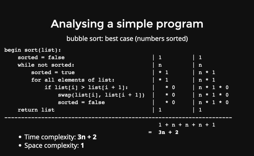
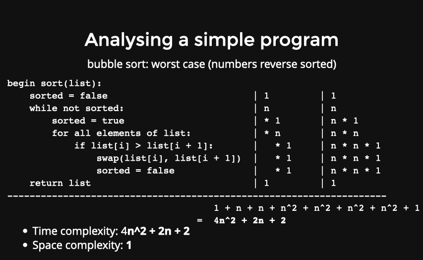
• The example programs discussed in the lectures use a constant amount of memory regardless of the increasing time taken to compute their equally increasing input sizes.

There is no syntax for pseudocode - a middle step between understanding and coding a problem up.

Theoretical Performance Analysis looks at pseudocode to evaluate the complexity of a program regardless of the hardware or software environment. This time complexity is expressed as an equation based on a variable ‘n’ where ‘n’ is the number of input elements.

Space Complexity (will be looked at later in the course): How much memory does this program use? How many bytes does it need to actually run?

• It doesn’t depend on n.

‘Constant time’: When your algorithm is not dependent on the input size n, it is said to have a constant time complexity. This means that the run time will always be the same regardless of the input size.

• log*n grows slower than any kind of n

<u>Time complexity describes how an algorithm scales (in terms of the amount of time taken) as the input size increases. Knowing the time complexity alone is not sufficient to determine how long an algorithm will take for a single given input size.</u>

Algoirthm Analysis:

Useful for looking at how programs scale, not necessarily how fast it runs.

Complexity is talking about asymptotic behaviour (we are describing the limiting behaviour).

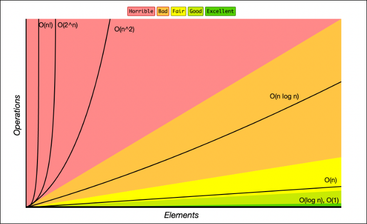
• The Upper Bound (O) of an algorithm's complexity describes how the algorithm's execution time changes with a change in the amount of data being processed in the operation, meaning that a more complex algorithm will often take an increasingly (often not linearly) long time to execute as the amount of data is increased.
• Asymptotes come into effect only when the input is large enough - this is when scale is considered. Complexity does not deal with small numbers, as they are unreliable and computers don’t deal with them as well as it does with big numbers.

Time complexity essentially asks for the tightest bound you can get ⇒ How quickly does your program run in the worst case?

Our computer can process an input of size 10 in one day. Now since the

algorithm runs in time O(2^n), our computer can process an input of size...

11 in 2 days

12 in 4 days

13 in 8 days

14 in 16 days

15 in 32 days

16 in 64 days

17 in 128 days

18 in 256 days

19 in 512 days

20 in 1024 days

Our computer will be able to process an input of size 19 in 1000 days.

The faster computer can process in one day what our computer can process

in 1000 days, since it is 1000 times faster. Hence the answer is 19.

Just add time in front of the compilation command:

gcc -Wall -Werror -O -o sum sum.c 
time gcc -Wall -Werror -O -o sum sum.c 
real    0m0.063s
user    0m0.026s
sys     0m0.000s

• real is the time taken on the clock to complete
• user is the time the CPU takes to process your program
• sys is the time taken by the OS for actions such as malloc, file open, file close, etc.

However the issues with this run time are:

• This requires implementation of the algorithm
• The run time can easily be influenced by the machine its being run on
• Because of point 2, we need to use the same machine and environment if we need to compare the run time between different algorithms implemented to resolve the same issue.

As such, we can use

Pseudocode --> writing code in very basic English terms

• This helps us evaluate its complexity without requiring a software or hardware environment.
• We can count the number of operations that occur in a program and then express the complexity based on the variable n (n being the number of input elements).

So how do we analyse a program? Here is an example:

We usually assume that primitive operations have 'constant time' but in reality they might require more than one step of processing (its whatever, we still consider them as constant time). Some primitive operations include:

• Indexing an array (getting/setting)
• Comparisons (equality, relational)
• Variable assignment

• difficulty based on:
  • solving – how hard is it to find/guess the correct answer? (time complexity, how many steps, etc.)
  • verifying – how hard is it to verify a given answer’s correctness?
• polynomial time problem = easy problems (table above)
• non-deterministic polynomial time problem = algorithm used to solve hard problems that can’t be solved for large data sets by standard computers
  • can only be solved in reasonable amount of time by theoretical computer that can simulate multiple possibilities at same time OR guess perfect answer immediately
• P vs. NP vs. NP-complete
  • P = polynomial
    • can be solved/verified in polynomial time
    • e.g. n, n^2, log(n), sqrt(n)
  • NP = non-deterministic polynomial
    • can be solved in non-deterministic polynomial time (by theoretical computers)
    • can be verified in polynomial time
    • e.g. n!, k^n, hamiltonian paths
  • NP-complete
    • can be solved only in non-deterministic polynomial time
    • can be verified in polynomial time
  • (NP-hard)
    • can only be solved in non-deterministic polynomial time
    • can only be verified in polynomial time

(12)

the algorithm with higher growth rate 
not only solves a smaller problem in a given time in the first place, 
it also receives less of a speedup from a faster computer.
=====================================================================================
a.)
int cmp(int a, int b) {
    return (a-b); 
}  
void sort(int a[], int n) { 
    int i, j, min; 
    for (i = 0; i < n-1; i++) { 
        min = i; 
            for (j = i+1; j < n; j++) {  
                // (a[j] < a[min]) 
                if (cmp(a[j],a[min]) < 0) 
                    min = j; 
                } 
                int t = a[min]; a[min] = a[i]; a[i] = t; 
            } 
} 
the cmp() function will be invoked n*(n-1)/2 times for an array of length n.
#####################################################################################
b.)

For input size = 1000, it will take 1 day
Time taken = C(10n)
1 = C*(101000)
C = 1/(101000)
--------------------------------------
For a faster computer(1000 times faster)
C' = (C/1000) = (1/(1000 * 101000)) = 1/(101003)
1 = C'(10N)
1 = (1/(101003))* (10N)
10N = (101003)
N = 1003
######################################################################################
c.) similar to above 

Suppose that a particular algorithm has time complexity n^2 and that executing an implementation of it on a particular machine 
 takes t seconds for $n$ inputs. Now suppose that we are presented with a machine that is 64 times as fast.
 How many inputs could we process on the new machine in t seconds?  (8n) 

 If you had a second program whose growth rate is 2^n
    and for which the original computer could run a problem of size 1000 in an hour, 
    than a machine ten times faster can run a problem only of size 1003 in an hour! 
    Thus, an exponential growth rate is radically different 
than the other growth rates shown 
######################################################################################
d.)
int i, j, k = 0;for (i = n / 2; i <= n; i++) 
 for (j = 2; j <= n; j = j * 2) 
 k = k + n / 2;                               O(nLogn)


for(var i=0;i<n;i++)
 i*=k                                         O(logkn)


for(int i=0;i<n;i++)
    for(int j=0;j<i;j++)                       n(n-1)

 int i = 1, s = 1;
    while (s < n) {
        s = s + i;
        i++;                                   sqrt(n)
######################################################################################
e.)
            insertion        deletion        search
BST :         O(h)/O(n)        O(h)/O(n)        O(h)/O(n)
AVL :         O(logn)          O(logn)          O(logn)
Stack:        O(1)             O(1)             O(n)
Queue:        O(1)             O(1)             O(1)
Heap:         O(logn)          O(logn)          O(n)
AoE:          O(E)             O(E)             O(E)
AoM(dense):   O(1)             O(1)             O(1)
AoL(sparse):  O(v)             O(v)             O(v)

Prims:        O(ElogV)
Kruskal:      O(ElogE)
Dijkstra:     O(V+E) AoL    O(v^2 logV) AoM // binary heap
BST join:     O(m) // height of right tree
######################################################################################
S: stability    A: adaptivity 

Bublesort(S,A):    O(n^2)        Insertion(S,A):    O(n^2)    
Selection(nil):    O(n^2)
Merge(S):          O(nlogn)      Qucik(nil):     O(nlogn)

Quiz question: An O(n^2) algorithm takes about 0.3 seconds to process 1000 numbers. Approximately how long will it take to process 10000 numbers?

Answer with solution: An O(n^2) algorithm will take approximately 10^2 = 100 times longer for an input size that is 10 times bigger. Therefore the algorithm would take 100 x 0.3 = 30 seconds to process 10000 numbers.

Worst case time complexities of data structures